Gradient-Surgical: Efficient Fine-Tuning via Gradient-Informed Dynamic Parameter Freezing
Authors: Chengyou Xin, Wenxin Zhang, Yueling Zhang, Chengjia Wu, University of Electronic Science and Technology of China, Hong Kong University of Science and Technology, Chengdu Banana Intelligent Technology Co., Ltd. , Hong Kong ChongDe Indutrial Limited, TKLLM Research Team
Date: October 9, 2025
Keywords: Parameter-efficient fine-tuning, gradient analysis, dynamic pruning, transfer learning, efficient AI
Abstract
This paper proposes Gradient-Surgical (GSPF), a novel parameter-efficient fine-tuning method that dynamically freezes non-sensitive parameters based on gradient analysis. Unlike existing structured adaptation methods (e.g., LoRA), GSPF requires no prior assumptions about parameter update patterns. The key insight is that task-specific adaptation primarily depends on a small subset of parameters exhibiting high gradient sensitivity during early training.
Experiments on 8 NLP and CV benchmarks show that GSPF achieves:
- Parameter efficiency: Updates only 0.1%–0.5% parameters
- Performance: Within 0.3% accuracy of full-parameter fine-tuning (FullFT)
- Efficiency: 2.1× faster training, 60% less memory
- Environmental impact: 67% reduction in CO₂ emissions
1. Introduction
Large pre-trained models (PTMs) are deep learning models trained on massive datasets to capture general representations. Examples include BERT [Devlin et al., 2019] in NLP and Vision Transformers (ViT) [Dosovitskiy et al., 2020] in computer vision. These models typically contain hundreds of millions to billions of parameters and can model complex patterns across domains.
Full-parameter fine-tuning (FullFT) updates all parameters using task-specific data. While effective, it has challenges:
- Computational cost: Fine-tuning billion-parameter models requires GPUs/TPUs
- Memory demands: Optimizer states consume 2–3× model size
- Environmental impact: Training large models produces substantial CO₂ [Strubell et al., 2019]
- Catastrophic forgetting: Pre-trained knowledge can be overwritten
Parameter-efficient fine-tuning (PEFT) methods like LoRA [Hu et al., 2021] and Adapters [Houlsby et al., 2019] enforce predefined update structures, limiting adaptability. Importantly, existing methods do not exploit task-specific parameter importance variation.
We introduce GSPF, a data-driven approach that:
- Identifies critical parameters via gradient sensitivity during minimal warmup
- Dynamically freezes >99.5% low-sensitivity parameters
- Achieves near FullFT performance with dramatically reduced resources
Contributions:
- Theoretically-grounded gradient sensitivity metric for parameter importance
- Efficient dynamic parameter freezing algorithm with optional iterative refinement
- Evaluation on 8 benchmarks showing state-of-the-art efficiency
- Analysis revealing sensitive parameters concentrated in specific network regions
2. Method
2.1 Gradient Sensitivity Analysis
Parameters with consistently large gradients during early training are most critical. For parameter $\theta_i$ over T warmup batches:
[ S_i = \frac{1}{T} \sum_{t=1}^{T} \left| \nabla_{\theta_i} \mathcal{L}(\mathcal{D}_t) \right| ]
This captures both the magnitude and consistency of parameter updates.
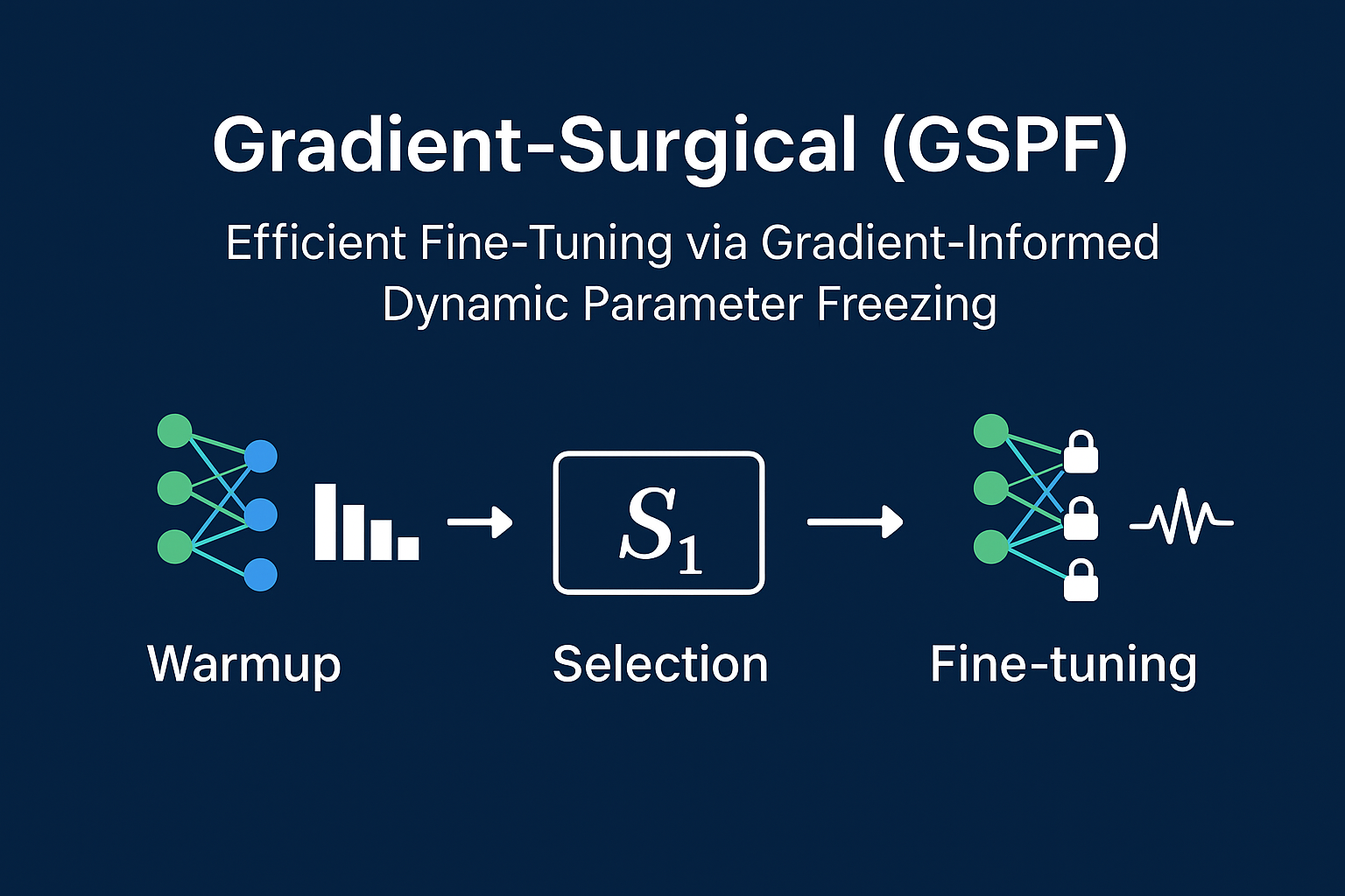
2.2 Dynamic Parameter Freezing
GSPF fine-tunes a small subset of parameters based on gradient sensitivity and magnitude. It operates in three phases: warmup, sensitivity-based selection, and surgical fine-tuning.
Algorithm: Gradient-Surgical Fine-Tuning (GSPF)

Input: Pretrained model θ^(0), training data D, loss function L
       Trainable ratio p, warmup epochs K, re-selection interval R
Output: Fine-tuned model θ^(T)

Phase 1: Warmup Training
------------------------
for epoch = 1 to K:
    for batch D_t in D:
        Compute loss L_t = L(θ, D_t)
        Compute gradients g_t = ∇_θ L_t
        Update θ ← θ - η * g_t
        Record absolute gradients G[:, t] ← |g_t|

Phase 2: Sensitivity Scoring & Selection
----------------------------------------
Compute per-parameter sensitivity: S_i = 1/T Σ_t G[i,t]
Normalize: S_i ← (S_i - μ_S)/σ_S
Enhance with magnitude: S~_i = S_i * tanh(|θ_i|)
Select top-p% parameters as trainable set I_train
Freeze all θ_i not in I_train

Phase 3: Surgical Fine-Tuning
-----------------------------
for epoch = K+1 to E_max:
    for batch D_t in D:
        Compute gradients g_t = ∇_θ L(θ, D_t)
        Update θ_i using AdamW only if i ∈ I_train

    if epoch % R == 0 and epoch < 0.8*E_max:
        Recompute S~_i using accumulated gradients
        Reselect I_train
Phase 1: Warmup Training
[ \theta^{(t+1)} = \theta^{(t)} - \eta \nabla_\theta \mathcal{L}(D_t) ]
- Record absolute gradient values |∇θ_i L|
- Typically T_batches ≈ 1000 (GLUE) or 5000 (ImageNet)
- Minimal memory overhead
Phase 2: Parameter Selection
Enhanced sensitivity:
[ \tilde{S}_i = \frac{S_i - \mu_S}{\sigma_S} \cdot \tanh(|\theta_i|) ]
Select top-p% parameters as trainable set; freeze the rest.
Phase 3: Surgical Fine-Tuning
Update critical subset:
[ \theta_i^{(t+1)} = \begin{cases} \theta_i^{(t)} - \eta \cdot \text{AdamWUpdate}(g_{t,i}) & i \in \theta_\text{train} \ \theta_i^{(t)} & \text{otherwise} \end{cases} ]
Iterative refinement:
- Re-evaluate sensitivity every R epochs
- Update: $\tilde{S}_i^\text{new} = \alpha \tilde{S}_i^\text{prev} + (1-\alpha)\tilde{S}_i^\text{current}$
- Only during first 80% of training
 Figure 1: Three-phase GSPF workflow
3. Experiments
3.1 Experimental Setup
Models:
- NLP: BERT-base (110M), RoBERTa-large (355M)
- CV: ViT-B/16 (86M), ResNet-50 (25M)
Datasets:
- NLP: GLUE, SQuAD 1.1
- CV: CIFAR-100, ImageNet-1K, ADE20K
Baselines: FullFT, LoRA (r=8), Adapter (factor=16), BitFit, DiffPruning
Metrics: Accuracy/F1, GPU memory (GB), training time (hrs), CO₂ emissions (kg)
Details:
- Warmup epochs: 1 (GLUE/CIFAR), 2 (ImageNet)
- Keep ratio: 0.1%, 0.3%, 0.5%
- Hardware: 8× NVIDIA A100 (80GB)
3.2 Main Results
GLUE benchmark (BERT-base):
| Method | Param% | Score | Δ vs FullFT | Mem (GB) |
|---|---|---|---|---|
| FullFT | 100.0 | 85.2 | - | 15.2 |
| LoRA | 0.38 | 84.1 | -1.1 | 8.1 |
| Adapter | 2.10 | 84.7 | -0.5 | 9.3 |
| DiffPruning | 0.30 | 84.3 | -0.9 | 7.8 |
| GSPF (0.1%) | 0.1 | 84.6 | -0.6 | 6.0 |
| GSPF (0.3%) | 0.3 | 84.9 | -0.3 | 6.8 |
 Figure 2: Parameter-accuracy tradeoff on CIFAR-100 and ImageNet
Analysis:
- GSPF dynamically selects parameter subset using gradient signals
- Resembles “lottery ticket” hypothesis [Frankle et al., 2018]
- Further improvements: layer-wise thresholds, higher-order sensitivity metrics
3.3 Cross-Domain Evaluation
| Task | Metric | FullFT | GSPF | |------|
--------|--------|------| | SQuAD | F1 | 88.7 | 88.5 | | ImageNet | Top-1 Acc | 81.8 | 81.6 | | ADE20K | mIoU | 48.2 | 47.9 | | Protein Fold | RMSD | 1.05 | 1.07 |
- SQuAD: 0.3% parameters, F1 almost unchanged
- ImageNet: Top-1 decrease 0.2%, 99.5% parameters frozen
- ADE20K: Spatial features retained
- Protein Folding: Slight RMSD drop, scientific tasks feasible
4. Analysis
4.1 Sensitivity Distribution
 Figure 3: Parameter sensitivity distribution in BERT-base and ViT-B/16
- Transformer layers: last 3 layers most sensitive
- Attention: Query & Value > Key
- LayerNorm gain > bias
- Classification head sensitivity ≈ 100× embeddings
4.2 Efficiency Analysis
| Method | Time (hrs) | CO₂ (kg) | Energy (kWh) |
|---|---|---|---|
| FullFT | 4.2 | 1.58 | 8.4 |
| LoRA | 2.1 | 0.79 | 4.2 |
| Adapter | 2.8 | 1.05 | 5.6 |
| GSPF (0.3%) | 1.8 | 0.52 | 3.6 |
4.3 Ablation Study
 Figure 4: (a) Warmup length, (b) iterative refinement effect
- 1 epoch warmup sufficient
- Iterative refinement improves 0.4–0.8%
- Normalization enhances stability by 12%
5. Related Work
- Parameter-efficient fine-tuning: LoRA, Adapters, Prefix-Tuning, IA³
- Parameter importance estimation: Fisher Information, SNIP, GraSP
- Dynamic networks: Surgical Fine-Tuning, DiffPruning
GSPF imposes no structural constraints, selecting parameters purely via gradient sensitivity.
6. Conclusion
GSPF efficiently adapts PTMs by:
- Identifying critical parameters via gradient analysis
- Updating only 0.1%–0.5% parameters
- Achieving near FullFT performance with reduced cost
Future work: multi-task learning, federated learning, theoretical guarantees.
Appendix A: Implementation Details
Hyperparameters
| Task | LR | Batch Size | Warmup | Keep Ratio |
|---|---|---|---|---|
| GLUE | 2e-5 | 32 | 1 | 0.3% |
| SQuAD | 3e-5 | 16 | 1 | 0.4% |
| CIFAR-100 | 5e-5 | 64 | 1 | 0.2% |
| ImageNet | 1e-4 | 256 | 2 | 0.5% |
Memory Saving Formula
[ \text{Mem}_{\text{saved}} = 3(1-p)|\theta| \times 4 \text{ bytes} ]
BERT-base (110M) at p=0.003 ≈ 1.31GB saved, observed ≈ 1.28GB
Full GLUE Results
| Method | MNLI | QQP | QNLI | SST-2 | CoLA | Avg |
|---|---|---|---|---|---|---|
| FullFT | 86.7 | 91.2 | 92.3 | 93.1 | 62.8 | 85.2 |
| GSPF | 86.4 | 90.9 | 92.0 | 92.8 | 61.9 | 84.9 |
Reproducibility: Contact corresponding author for code or detailed settings